Unsupervised ANNs Algorithms and TechniquesTechniques and algorithms which are used in unsupervised ANNs involve self-organizing maps, restricted Boltzmann machines, autoencoders, etc. Self-organizing maps:Self-organizing maps are a basic type of artificial neural network whose growth depends on unsupervised learning procedures and exploitation of the similarities between data. Self-organizing maps are biologically inspired by topographically computational maps that are learned by self-organization of its neurons. This motivation originated from how different inputs are organized into topographic maps in human brains. Self-organizing maps, unlike supervised ANN, comprises of input and output neurons with no hidden layers and are developed in such a way that only one of the output neurons can be activated. It concludes competitive learning, a procedure where all the output neurons compete with each other. The winner of such competition is fired and referred to as the winning neuron. With the search of the output neurons having sets of weights which characterize their coordinates in the input space, one method for understanding the competition between output neuron is by computing the value of the discriminant function, typically Euclidean distance between them and the component vector of the current sample into the input. Selecting neurons, from a group of neurons which are situated at the nodes of a lattice, are turned into numerous input patterns, organizing themselves, and forming a topographic map over the lattice structure. The coordinates of the neurons show statistical representation in the input structures when provided with input signals. Self-organizing maps, as their name suggests provide a topographic map that internally portrays the statistical features in input patterns of the supplied input. Initialization, competition, adaptation, and cooperation are the significant components involved with the self-organization of neurons. At the initial stage, randomly selected small values are initially allocated as weights of output neurons. Output neurons would then compete with each other by comparing the values of the discriminant function. The output neuron that limits the values of the discriminant function is selected as the winner and has its weights updated such that it is moved nearer to the present observation. There is a cooperation between the winning neuron those in its neighborhood (characterized by a radius) because not only its weights updated, but also the weights of the predefined neighborhood are updated as well, with the winning neurons getting relatively higher updates towards the input vector. This collaboration is inspired by lateral connections among groups of excited neurons in the human brain. The updated weight received by neighboring neurons is a function of the lateral distance among them and winning neurons with the nearest and farthest neurons accepting the highest and lowest weight update, respectively. The weights are updated for effective unsupervised classification of data. The data behind this is the need to improve the similarity between a unit that best matches the training input. An undirected graphical model usually referred to as the best matching unit, and those in a neighborhood to the input. The five phases associated in self-organized maps algorithm are sampling, initialization, finding the neuron whose weight vector best matches the input vector, updating the weights of the winning neuron, and those in the neighborhood using the given equation, and returning the sampling stage until ni(number of inputs) progressions can be implemented in the feature map. Kohonen network is a kind of self-organized map. ∆wji = ŋTj I(X) (t)(xi- wji) 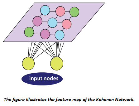 The Kohonen networks feature map is shown in the figure. Self-organizing maps artificial neural networks are generally applied for clustering and brain-like feature mapping. They are appropriate for application in the areas of exploratory data, statistical, biomedical, financial, industrial, and control analysis. Restricted Boltzmann machines:Boltzmann machines (BMs) have been introduced as bi-directionally connected networks of hypothetical processing units, which can be interpreted as neural network models. Boltzmann machines can be used to learn significant aspects of an unknown probability distribution based on samples from the distribution. Generally, this learning procedure is difficult and tedious. However, the learning issue can be simplified by imposing limitations on the network topology, which leads us to restricted Boltzmann machines. A restricted BM is a generative model representing a probability distribution. Given a few observations, the training data, learning a BM, implies changing the BM parameters to such that the probability distribution represented by the BM fits the training data. Boltzmann machines comprise of two types of units, visible and hidden neurons, which can be arranged in two layers. The visible units establish the primary layer and correspond to the components of observations. For example, one visible unit for each pixel of a digital image. In the hidden units, model dependencies lie between the components of observations. For example, dependencies between pixels in images. They can be viewed as non-linear element indicators. 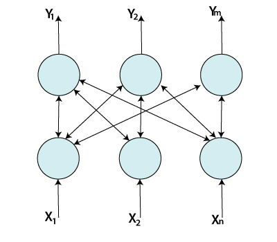 Boltzmann machines can also be viewed as specific graphical models, more precisely undirected graphical models, also known as Markov random fields. The embedding of BMs into the structure of probabilistic graphical models gives quick access to an abundance of hypothetical outcomes and well-developed algorithms. Computing the probability of an undirected model or its gradient for inference is generally computationally comprehensive. Hence, sampling-based techniques are utilized to estimate the probability and its gradient. Sampling from an undirected graphical model is usually not simple, but form RBMs Markov Chain Monte Carlo (MCMC) techniques are easily applicable in the form of Gibbs sampling. 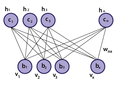 A restricted Boltzmann machine (RBM) is a Markov random field (MRF) related to a two undirected graph illustrated in the given figure. It includes x visible units V = (V1,…, Vx) to show data and n hidden units H = (H1,…, Hn) to catch observed variables. In binary RBMs, our focus on the random variables (V, H) takes values (V, H) ∈ {0,1}x+n and the joint probability distribution under the model given by the Gibbs distribution P(V, H) = 1/z e-E(v,h) having the energy function.  For all i ∈ {1, ..., n} and j ∈ {1, ..., x}, Wij is a real-valued weight connected to the edge between units Vj and Hi, and Bj and Ci are real-valued bias terms connected to the jth visible and the ith hidden variable, respectively. The graph of an RBM has an only association between the layer of hidden and visible variables but not between two variables of a similar layer. In terms of probability, it implies that the hidden variables are independent, given the state of the visible variables and vice versa. Autoencoders: An autoencoder is a kind of neural network that is prepared to attempt to copy its input to its output. Internally, it has a hidden layer that portrays a code used to represent the input. Autoencoder is ANNs with asymmetric structures, where the middle layer represents an encoding of the input data. Autoencoder is prepared to reconstruct their input onto the output layer while confirming certain limitations that keep them from copying the data along with the network. Although the term autoencoder is the most popular these days, they were also called auto-associative neural networks, diabolo network, and replicator neural networks. 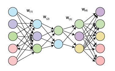 The basic structure of an autoencoder is shown in the figure given below. It incorporates an input p that is mapped onto the encoding b through an encoder, represented as function F. This encoding is mapped to be a recreation r utilizing a decoder, represented as function Z. This structure is captured in a feedforward neural network. Since the goal is to reproduce the input data on the output layer, both p and r have a similar dimension. p can have higher-dimension or lower dimensions, depending upon the desired properties. The autoencoder can also have various layers as required, generally placed symmetrically in the encoder and decoder. Such neural architecture can be seen in the figure given below. 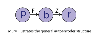 Next TopicBrain-State-in- a Box Network |