Spaceship Titanic Project using Machine Learning - PythonThe Spaceship Titanic Problem is an advanced version of the basic Titanic Survival Problem which machine-learning lovers must face once and predicted a person's survival chances. Problem Statement of the Spaceship Titanic ProjectIn this project, a spaceship contains several people going into Space for a trip. Due to technical problems, many of them are transported to another planet. Using various machine learning algorithms; we have to predict the people who will be transported to another planet or remain on the same spaceship. Approach to Solve the Spaceship Titanic ProblemStep 1: Libraries and Dataset The first step is to import the required libraries, including numpy, pandas, matplotlib, sklearn, etc., for building and analyzing a machine learning model. Then, we will load the dataset for the Spaceship Titanic Problem and store it in the pandas data frame. Step 2: Data Cleaning After loading the dataset, we will clean the data. Data Cleaning includes checking the null values in the data, replacing the null values with some values (it may be an average of other values or a 0), and checking outliers before proceeding further. We can analyze the data with the help of charts. The null values can be checked using the describe() method. Step 3: Feature Engineering Now, we will select features to build our model and predict the outcome. We will gather significant information by comparing different features. Step 4: Exploratory Data Analysis We will perform exploratory data analysis to study the relationship between different features. We will visualize these relations with different charts and graphs like pie charts and bar graphs to study the correlation. Step 5: Splitting the dataset We will split the data set into training and testing data sets using the train_test_split model and normalize the data using Standard Scaler. Step 6: Training of the model Now, we will train our data set using different machine learning algorithms like logistic regression, SVC, and XGBClassifier and check their accuracy. Step 7: Choosing the best model We will choose the model with the highest accuracy. Step 8: Confusion matrix and Validation data Using the machine learning model with the best performance, we will print the confusion matrix and validation data. Step 9: Prediction Using the machine learning model created, we can predict whether the person will be transported to the new planet or remain on the same. Now, let's begin the implementation of the Spaceship Titanic Problem.
We have imported the required libraries like numpy, pandas, matplotlib, sklearn packages like train_test_split, different algorithms, etc. Now we will load the dataset. Output: 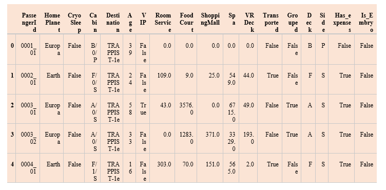 We have read the dataset and stored it in the data frame. We have printed the top 5 records using the head() function. Data Preprocessing of the datasetOutput: (8693, 18) We will look at the data more deeply. Output:
Using the shape() function, we can check the dataset's number of rows and columns. The info() function will tell us if there is any null value in the dataset, along with the data type of each column. Looking into the above output, we can see many null values in the dataset. Now we will get the descriptive statistical view of the dataset using the describe() method. It tells about the count, unique values, top, and frequency. Output: 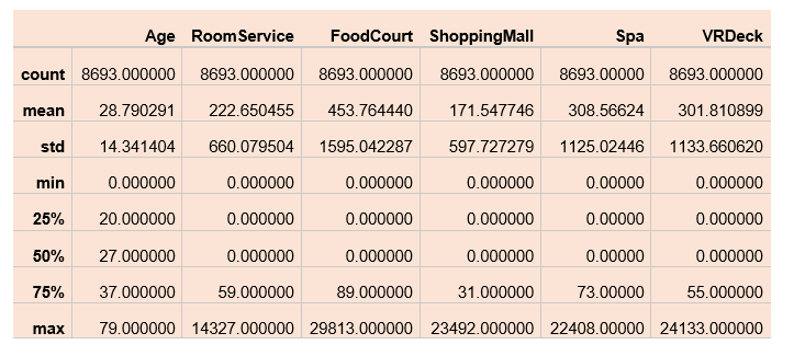 One of the simplest ways to replace the null values is to impute null by mean in the case of continuous data and mode in the case of categorical values. Still, in this case, we will try to examine the relationship between independent features and then use them to impute the null values cleverly. Output: 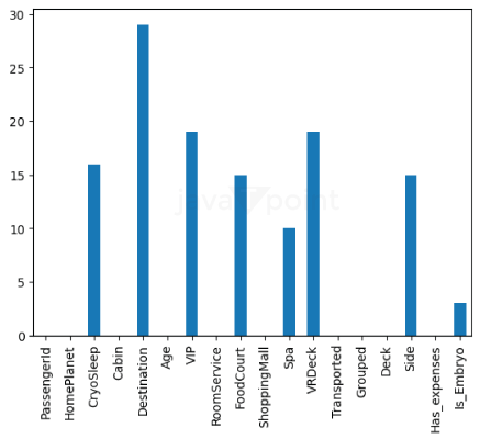 clm = data.loc[:,'RoomService':'VRDeck'].columns
data.groupby('VIP')[clm].mean()
Output:  We can see that VIPs have more expenses than Non-VIP people. data.groupby('CryoSleep')[clm].mean()
Output: Passengers in CryoSleep are restricted to their rooms and suspended in animation for the voyage. Thus, they are unable to spend money on onboard amenities. As a result, when CryoSleep equals True, we may enter 0. We will replace the null values using the relation between VIPs and their expenses. We have filled the null values in the VIP column with different values. After observing the outliers, we will fill the age null values with the mean. For this, we will plot a boxplot. Output: 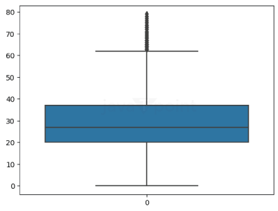 With the help of this box plot, we can calculate the mean and then replace the null value. As we have filled the null values of the age values. Now we will check again for the null values, if any. Output: 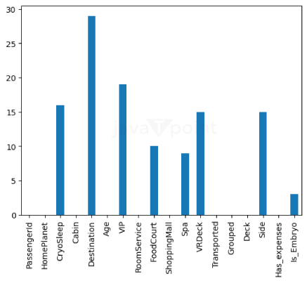 From this plot, we have noticed more null values. Let's replace those. Output: 0 Finally, we have removed all the null values from the dataset. Feature EngineeringAs we have preprocessed our data, it's time to select features and add the data to it. We will add some features to get more insights from the data and make more accurate predictions. Output: 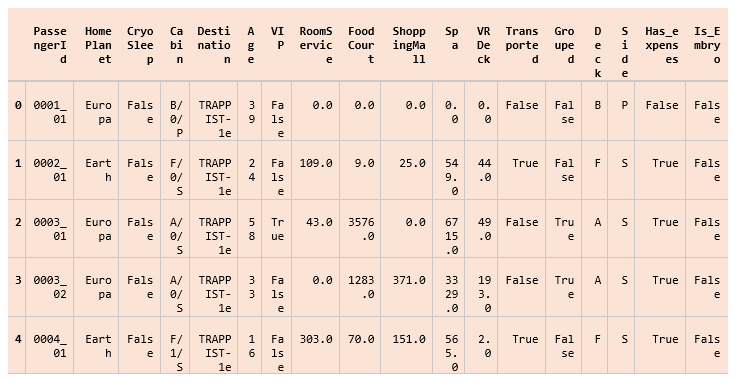 We can see that there are some features with combined data. We will separate the data and make some new features out of it. We have split the PassengerID feature into RoomNo and PassengerNo. We have split the Cabin feature into three new columns F1, F2, and F3. And dropped the column Cabin. We have combined different columns, like RoomService, FoodCourt, etc., into the LeseaureBill. Exploratory Data AnalysisWe have transformed different features. Now, it's time to visualize and analyze the data. Output: 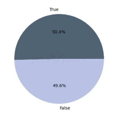 From this pie chart, we can see that both the classes have equal distribution. Thus, it will be easy to train the model. Output: 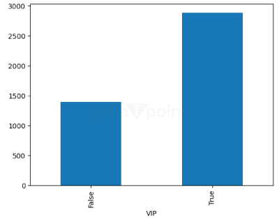 Output: 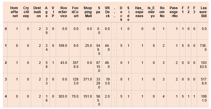 5 rows × 22 columns Output: 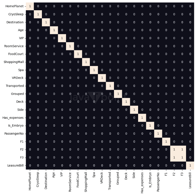 Training the ModelOutput: ((7823, 21), (870, 21)) We split the dataset into training and testing data sets, with 90% training and 10% test data. We have now scaled our dataset using the Standard Scaler. Now, we will check the training and validation accuracy of different machine-learning algorithms. Output: LogisticRegression() :
Training Accuracy : 0.878723950049363
Validation Accuracy : 0.8617140797897147
XGBClassifier(base_score=None, booster=None, callbacks=None,
colsample_bylevel=None, colsample_bynode=None,
colsample_bytree=None, early_stopping_rounds=None,
enable_categorical=False, eval_metric=None, feature_types=None,
gamma=None, gpu_id=None, grow_policy=None, importance_type=None,
interaction_constraints=None, learning_rate=None, max_bin=None,
max_cat_threshold=None, max_cat_to_onehot=None,
max_delta_step=None, max_depth=None, max_leaves=None,
min_child_weight=None, missing=nan, monotone_constraints=None,
n_estimators=100, n_jobs=None, num_parallel_tree=None,
predictor=None, random_state=None, ...) :
Training Accuracy : 0.9891161010670031
Validation Accuracy : 0.8838555136303896
SVC(probability=True) :
Training Accuracy : 0.9049843360030313
Validation Accuracy : 0.8660093483698648
We can see that the Logistic Regression has 87% training accuracy and 86% validation accuracy. The XGBClassifier has 98% training accuracy and 88% validation accuracy. The SVC has 90% training accuracy and 86% validation accuracy. The XGB classifier has the, highest accuracy thus, is the best fit for the model. Evaluating the ModelOut of the three machine learning models, the XGB classifier has the best performance. Now we will make a confusion matrix and print the predictions. Output: array([0, 0, 0, 0, 0, 0, 0, 1, 1, 0, 0, 0, 0, 0, 1, 0, 1, 1, 1, 0, 0, 1,
1, 1, 1, 0, 1, 0, 1, 0, 1, 0, 1, 0, 0, 0, 0, 1, 0, 0, 0, 1, 0, 1,
0, 0, 1, 0, 1, 0, 0, 1, 1, 1, 0, 1, 1, 1, 0, 0, 1, 0, 0, 1, 0, 1,
1, 1, 0, 1, 0, 1, 0, 1, 0, 0, 1, 0, 0, 0, 1, 1, 0, 1, 0, 0, 0, 0,
1, 0, 0, 1, 0, 0, 0, 1, 1, 0, 1, 0, 1, 0, 1, 1, 1, 0, 0, 0, 0, 1,
1, 0, 1, 0, 1, 0, 1, 1, 0, 0, 0, 0, 1, 0, 1, 1, 0, 1, 0, 0, 1, 0,
0, 0, 0, 0, 1, 1, 1, 1, 1, 1, 1, 1, 0, 1, 1, 0, 0, 0, 1, 0, 1, 1,
1, 1, 0, 1, 1, 0, 0, 0, 0, 1, 0, 0, 0, 1, 0, 1, 1, 1, 0, 0, 0, 1,
1, 0, 0, 0, 1, 0, 0, 1, 0, 1, 1, 0, 0, 0, 1, 1, 0, 0, 1, 0, 0, 0,
1, 0, 1, 0, 1, 1, 0, 1, 0, 0, 1, 1, 1, 1, 1, 0, 1, 1, 0, 0, 1, 0,
1, 1, 0, 1, 1, 0, 0, 1, 0, 0, 1, 1, 1, 0, 1, 0, 1, 1, 0, 1, 1, 1,
0, 0, 0, 1, 1, 0, 0, 0, 1, 1, 0, 0, 1, 0, 1, 0, 0, 0, 0, 1, 0, 0,
0, 1, 1, 1, 1, 0, 0, 1, 1, 0, 0, 0, 1, 0, 0, 0, 0, 1, 1, 0, 0, 1,
1, 0, 1, 0, 0, 0, 0, 0, 0, 1, 0, 1, 0, 1, 0, 1, 1, 0, 0, 0, 0, 1,
0, 0, 1, 1, 0, 1, 0, 0, 0, 0, 0, 1, 1, 0, 1, 1, 1, 0, 1, 0, 0, 1,
1, 1, 1, 0, 1, 0, 0, 0, 1, 0, 1, 0, 1, 0, 1, 0, 1, 1, 1, 1, 0, 1,
1, 0, 0, 1, 1, 0, 1, 1, 1, 0, 1, 1, 0, 0, 0, 1, 0, 0, 1, 1, 0, 1,
0, 1, 0, 0, 1, 0, 0, 1, 0, 1, 0, 0, 0, 0, 0, 0, 0, 0, 1, 1, 1, 1,
1, 1, 1, 1, 1, 1, 1, 1, 0, 0, 0, 0, 0, 0, 1, 0, 1, 1, 0, 0, 1, 0,
1, 1, 1, 0, 0, 1, 1, 1, 1, 1, 1, 1, 0, 0, 1, 0, 1, 1, 0, 1, 0, 1,
0, 1, 1, 0, 0, 0, 0, 1, 0, 0, 1, 1, 1, 1, 0, 0, 0, 0, 0, 0, 0, 0,
1, 0, 0, 1, 0, 0, 1, 1, 1, 1, 1, 1, 1, 1, 0, 0, 1, 1, 0, 1, 0, 0,
1, 1, 0, 0, 0, 1, 1, 0, 0, 1, 1, 1, 0, 0, 0, 0, 0, 1, 1, 1, 0, 1,
1, 0, 0, 0, 0, 1, 1, 0, 0, 0, 1, 1, 0, 0, 1, 1, 0, 1, 1, 1, 1, 0,
1, 0, 0, 1, 1, 1, 1, 1, 1, 1, 0, 1, 1, 0, 0, 0, 0, 0, 0, 1, 1, 1,
0, 0, 1, 1, 1, 0, 0, 1, 1, 1, 0, 0, 0, 1, 1, 0, 1, 1, 1, 1, 1, 0,
1, 1, 1, 0, 1, 1, 1, 1, 1, 0, 1, 0, 0, 1, 1, 0, 0, 1, 0, 1, 0, 1,
1, 0, 1, 0, 0, 1, 0, 1, 0, 1, 0, 1, 0, 0, 1, 0, 0, 1, 1, 0, 1, 1,
1, 0, 1, 0, 1, 1, 1, 1, 1, 0, 0, 0, 0, 0, 1, 1, 0, 0, 1, 0, 0, 0,
0, 0, 1, 1, 0, 0, 0, 0, 1, 0, 0, 0, 1, 0, 0, 1, 1, 0, 0, 1, 0, 0,
0, 0, 0, 0, 1, 0, 0, 1, 1, 0, 1, 0, 1, 0, 1, 0, 1, 0, 1, 1, 1, 1,
0, 0, 0, 0, 0, 0, 0, 0, 1, 1, 0, 1, 1, 0, 1, 0, 1, 1, 1, 0, 1, 1,
0, 1, 0, 1, 0, 1, 1, 0, 0, 1, 0, 1, 0, 0, 0, 1, 1, 0, 0, 1, 1, 0,
0, 0, 1, 1, 0, 0, 1, 1, 1, 1, 1, 1, 0, 1, 0, 1, 0, 0, 0, 1, 0, 1,
0, 1, 0, 1, 1, 0, 1, 0, 0, 0, 0, 1, 0, 1, 0, 1, 1, 1, 0, 0, 1, 0,
0, 0, 0, 1, 0, 0, 1, 0, 1, 1, 0, 1, 1, 0, 0, 1, 0, 1, 0, 1, 0, 0,
1, 0, 1, 1, 0, 0, 0, 1, 1, 0, 0, 0, 0, 1, 0, 0, 1, 0, 0, 0, 1, 1,
1, 1, 1, 1, 0, 0, 0, 0, 1, 0, 1, 1, 1, 0, 1, 1, 0, 0, 0, 1, 1, 1,
1, 0, 0, 0, 1, 1, 1, 0, 1, 0, 1, 0, 0, 1, 1, 1, 1, 0, 0, 1, 0, 0,
1, 1, 1, 1, 1, 0, 1, 1, 1, 0, 1, 1])
The prediction 0 refers to False and 1 to True. Output: 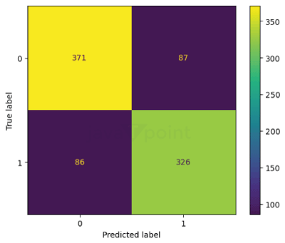 Output: precision recall f1-score support
0 0.82 0.79 0.80 458
1 0.78 0.80 0.79 412
accuracy 0.80 870
macro avg 0.80 0.80 0.80 870
weighted avg 0.80 0.80 0.80 870
Next TopicNaive Bayes algorithm in Python |