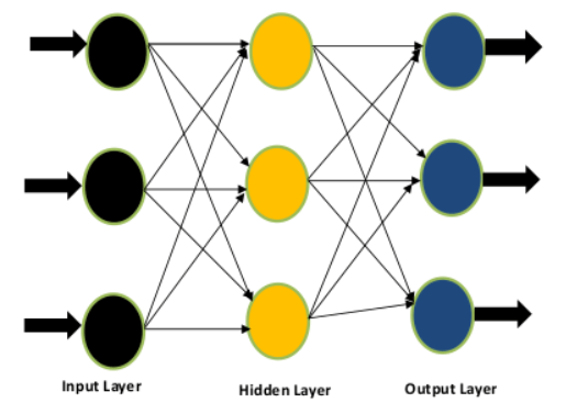
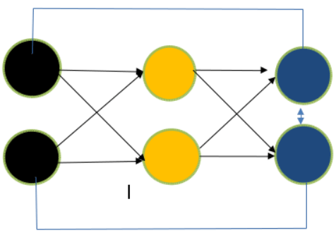
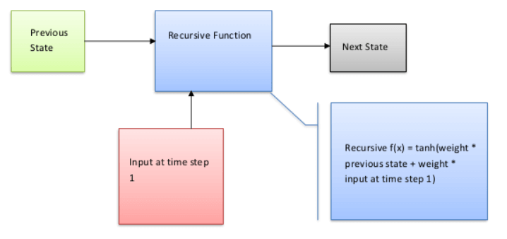
Difference Between Feed Forward Neural Network and Recurrent Neural NetworkFeed Forward Neural NetworkAn artificial neural network that feeds information forward lacks feedback between the input and the output. A network without cyclic connections between nodes can also be used to describe it. Let's look at it as a diagram.  You will see in the above Figure that there are three layers-the input, concealed layer, and output layer-and that information only flows in one direction. Due to the absence of backward flow, the moniker "feed-forward network" is appropriate. From output to input feedbackA subtype of artificial neural networks called recurrent neural networks, or RNNs, have ongoing communication between its input and output. It can be described as a network where nodes (found in the input layer, hidden layer, and output layer) are connected in a way that results in a directed graph. Let's examine it as a diagram.  The construction of the feed-forward neural network and the recurrent neural network are identical, except for feedback between nodes, as can be seen in the above image. This feedback will improve the data, whether they are self-neuronal or from output to input. RNN and Feed Forward Neural Networks vary from each other in yet another important way. The output of the previous state will be fed into the RNN as the input for the subsequent state (time step). With feed-forward networks, which deal with fixed-length input and fixed-length output, this is not the case. RNNs are, therefore, excellent for tasks requiring us to forecast the next character or word using our understanding of the preceding phrases, characters, or words. To learn more, please take a look at the sample below.  Let's give this Figure a textual description to understand its flow. RNN's internal memory allows it to memorize the input. It considers both the input it receives now and the past. It multiplies the previous weight input using the recursive function before using the tanh function to input a new weight at step 1. For a mathematical explanation of my concept, please examine the equation below. Recurrent Neural Network(RNN):Recurrent neural networks lead to an increase in complexity (RNN). They keep track of the output from processing nodes and include it in the model (they only did not pass the information in one direction). This is how the model is claimed to learn to anticipate the outcome of a layer. Each node in the RNN model serves as a memory cell, continuing calculation and operation execution when a network predicts something incorrectly. Through backpropagation, the system self-learns and keeps trying to generate the correct forecast. Pros:
Cons:
Vanishing Gradient issue in RNNLet's examine the definitions of vanishing gradient and explosive gradient. Understanding these two concepts will make it easier to comprehend the RNN challenge. Equations 3 and 4 must be used for these. In a disappearing gradient, d(e)/d(w) 1. The weight change will be minimal as a result. There will be little change in the weight if the new weight is calculated using equation (4), which causes the gradient to vanish. Let's now examine the exploding gradient problem. If d(e)/d(w) 1, the weight change will be considerable, increasing the new weight relative to the previous weight. This will cause the gradient problem to explode. If d(e)/d(w) 1, the weight change will be considerable, increasing the new weight relative to the previous weight. This will cause the gradient problem to explode. Two things influence the gradient's strength. Weight and activation function are the two. The product of several gradients is used to generate gradients for deeper layers (activation function). Let's discuss the issue of vanishing gradient in the context of RNN.  To determine the error, It will rely on the prior states, specifically the weights for e(t-2) and e. (t-1). The preceding weights (previous layers) must all be changed when the gradient (d()/d(w)) is backpropagated. The issue is that the gradient will grow as one approaches the cost function t but contract as one moves away from it. The output (y(t)) is unaffected by the gradient associated with e(t-2) during training. These crucial concepts are for understanding the vanishing gradient in RNN.
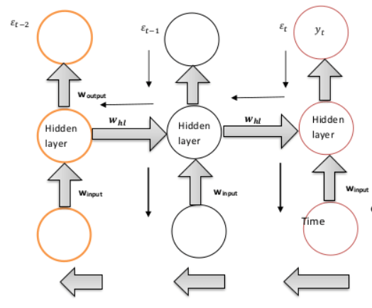
Another query that should cross your mind is why gradient is significant in the context above: The context above can be explained as follows: Gradient aids in learning. The learning rate increases as the gradient become steeper. Learning slows down when the gradient declines or gets smaller. Due to this issue, RNN is less than ideal for sequential modeling when memorizing deeper context. LSTM (Long Short-Term Memory), It addresses this problem and is covered in the section below. Next TopicFind Lower Insertion Point in Python |

We provides tutorials and interview questions of all technology like java tutorial, android, java frameworks
G-13, 2nd Floor, Sec-3, Noida, UP, 201301, India


